📖 正文内容
Pandas 简介
Pandas 库是机器学习四个基础库之一, 它有着强大的数据分析能力和处理工具。它支持数据增、删、改、查;支持时间序列分析功能;支持灵活处理缺失数据;具有丰富的数据处理函数;具有快速、灵活、富有表现力的数据结构:DataFrame 数据框和 Series 系列。
读写文本文件
- 文本文件是一种由若干行字符构成的计算机文件,它是一种典型的顺序文件。
- csv 是一种逗号分隔的文件格式,因为其分隔符不一定是逗号,又被称为字符分隔文件,文件以纯文本形式存储表格数据(数字和文本)。
1. 文本文件读取
read_csv(filepath_or_buffer, sep=',', header='infer', names=None, index_col=None, dtype=None, engine=None, nrows=None)
参数名称 | 说明 |
filepath | 接收 string。代表文件路径。无默认。 |
sep | 接收 string。代表分隔符。read_csv 默认为' , ',read_table 默认为制表符 '[Tab]'。 |
header | 接收 int 或 sequence。表示将某行数据作为列名。默认为 infer,表示自动识别。 |
names | 接收 array。表示列名。默认为 None。 |
index_col | 接收 int、sequence 或 False。表示索引列的位置,取值为 sequence 则代表多重索引。默认为 None。 |
dtype | 接收 dict。代表写入的数据类型(key:列名,values:数据格式)。默认为 None。 |
engine | 接收 C 或者 Python。代表数据解析引擎。默认为 C。 |
- sep 参数是指定文本的分隔符,如果分隔符指定错误,在读取数据的时候,每一行数据将连城一片。
- header 参数是用来指定列名,如果是 None 则会添加一个默认的列名。
- encoding 代表文件的编码格式,常用的编码有 utf-8、utf-16、gbk、gb18030、big5 等。如果编码指定错误,数据将无法读取,Ipython 解释器会报解析错误。
In [ ]
importpandasaspd
# 读取数据
data_txt = pd.read_csv('./text_similarity.txt', sep='\t')
# 查看数据
data_txt
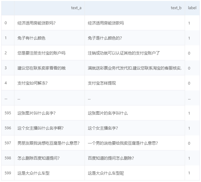
(运行项目后查看效果更佳)
In [ ]
# 读取数据
data_csv = pd.read_csv('./submit.csv', encoding='big5', header=0)
# 查看数据
data_csv
id value
0 id_0 5.174960
1 id_1 18.306214
2 id_2 20.491218
3 id_3 11.523943
4 id_4 26.616057
.. ... ...
235 id_235 41.266544
236 id_236 69.027892
237 id_237 40.346249
238 id_238 14.313744
239 id_239 15.770727
[240 rows x 2 columns]
2. 存储成文本文件
结构化数据通过 Pandas 中的 to_csv 函数实现以 csv 文件格式存储文件。
DataFrame.to_csv(path_or_buf=None, sep=',', na_rep='', columns=None, header=True, index=True, index_label=None, mode='w', encoding=None)
参数名称 | 说明 |
path_or_buf | 接收 string。代表文件路径。无默认。 |
sep | 接收 string。代表分隔符。默认为 ','。 |
na_sep | 接收 string。代表缺失值。默认为 ' '。 |
columns | 接收 list。代表写出的列名。默认为 None。 |
header | 接收 boolean。代表是否将列名写出。默认为 True。 |
index | 接收 boolean。代表是否将行名(索引)写出。默认为 True。 |
index_label | 接收 boolean。代表索引名。默认为 None。 |
mode | 接收特定 string。代表数据写入模式。默认为 w。 |
encoding | 接收特定 string。代表存储文件的编码格式。默认为 None。 |
注:下方操作会改变原有文件里的内容,因此我放置了一个对照组,work/text_similarity.txt和work/text_similarity2.txt在运行下方代码前的内容与格式是一致。
In [ ]
# 去掉注释‘#’后可运行
# data_txt.to_csv('./text_similarity2.txt', index=None, encoding='utf-8')
读写 Excel 文件
Pandas 提供了 read_excel 函数来读取 'xls'、'xlsx' 两种 Excel 文件。
1. 读取Excel 文件
pandas.read_excel(io, sheetname=0, header=0, index_col=None, names=None, dtype=None)
参数名称 | 说明 |
io | 接收 string。代表文件路径。无默认。 |
sheet_name | 接收 string 或 int。代表 excel 表内数据的分表位置。默认为0。 |
header | 接收 int 或 sequence。表示将某行数据作为列名。默认为 infer,表示自动识别。 |
names | 接收 int、sequence 或 False。表示索引列的位置,取值为 sequence 则代表多重索引。默认为 None。 |
index_col | 接收 int、sequence 或 False。表示索引列的位置,取值为 sequence 则代表多重索引。默认为 None。 |
dtype | 接收 dict。代表写入的数据类型(列名为 key,数据格式为 values)。默认为 None。 |
In [ ]
importpandasaspd
data_excel = pd.read_excel('./scores.xlsx', sheet_name='Sheet1')
# 查看Sheet1
data_excel
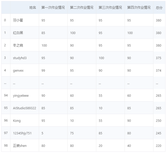
(fork 后查看效果更佳)
In [ ]
data_excel = pd.read_excel('./scores.xlsx', sheet_name='Sheet2')
# 查看Sheet2
data_excel
time state
0 2016-08-15 11:16:03 NaN
1 2016-08-15 11:28:56 NaN
2 2016-08-15 12:09:39 NaN
3 2016-08-15 12:24:47 NaN
4 2016-08-15 12:59:37 NaN
.. ... ...
94 2016-08-20 11:16:48 NaN
95 2016-08-20 11:23:58 NaN
96 2016-08-20 11:34:38 NaN
97 2016-08-20 11:45:59 NaN
98 2016-08-20 11:52:34 NaN
[99 rows x 2 columns]
2. 存储成 Excel 文件
to_excel 函数的语法格式如下:
DataFrame.to_excel(excel_writer=None, sheetname=None, na_rep='', columns=None, header=True, index=True, index_label=None, mode='w', encoding=None)
参数名称 | 说明 |
excel_writer | 指定存储文件的路径或使用现有的 Excel Writer。默认为 None。 |
sheet_name | 指定存储的 Excel Sheet 的名称。默认为 Sheet1。 |
na_sep | 接收 string。代表缺失值。默认为 ' '。 |
columns | 接收 list。代表写出的列名。默认为 None。 |
header | 接收 boolean。代表是否将列名写出。默认为 True。 |
index | 接收 boolean。代表是否将行名(索引)写出。默认为 True。 |
index_label | 接收 boolean。代表索引名。默认为 None。 |
mode | 接收特定 string。代表数据写入模式。默认为 w。 |
encoding | 接收特定 string。代表存储文件的编码格式。默认为 None。 |
注:下方操作会改变原有文件里的内容,下载到本地即可查看新内容。
In [ ]
# 去掉注释‘#’后可运行
# data_excel.to_excel('./scores.xlsx', index=None, sheet_name='test1')
DataFrame 的常用操作
- Series 可以看作特殊的 DataFrame 一列数据。Series 是一个一维的序列。
In [ ]
import pandas as pd
# 将列表里的元素,构建 Series
ser1 = pd.Series([1,2,'x'],index=['a','b','c'])
print(ser1)
# 将字典的键值对,构建 Series
ser2 = pd.Series({'a':[1,2,3],'b':['1','2','3']})
print(ser2)
a 1
b 2
c x
dtype: object
a [1, 2, 3]
b [1, 2, 3]
dtype: object
In [ ]
# 通过 DataFrame 构造数据框
d = [[1.0,2.2,3,4],[1,2,3,4],[7,8,9,0],[3,5,7,9]]
print(d)
df = pd.DataFrame(d)
print(df)
# index 修改行名称,columns 修改列名称
df = pd.DataFrame(d, index=['a','b','c','d'], columns=['A','B','C','D'])
print(df)
[[1.0, 2.2, 3, 4], [1, 2, 3, 4], [7, 8, 9, 0], [3, 5, 7, 9]]
0 1 2 3
0 1.0 2.2 3 4
1 1.0 2.0 3 4
2 7.0 8.0 9 0
3 3.0 5.0 7 9
A B C D
a 1.0 2.2 3 4
b 1.0 2.0 3 4
c 7.0 8.0 9 0
d 3.0 5.0 7 9
In [ ]
# 将字典变成数据框
d={'color':['blue','green','gold','red','grey'],
'object':['car','bus','van','boat','ship'],
'price':[1.2,2.3,3,4.5,5.6]}
frame = pd.DataFrame(d,index=['a','b','c','d','e'])
print(frame)
color object price
a blue car 1.2
b green bus 2.3
c gold van 3.0
d red boat 4.5
e grey ship 5.6
In [ ]
# 生成缺失值的 DataFrame
pd.DataFrame(index=['1','2'], columns=['b','c'])
b c
1 NaN NaN
2 NaN NaN
In [ ]
# 生成全零的 DataFrame
pd.DataFrame(0, index=['1','2'], columns=['b','c'])
b c
1 0 0
2 0 0
函数 | 返回值 |
values | 元素 |
index | 索引 |
columns | 列名 |
dtypes | 类型 |
size | 元素个数 |
ndim | 维度数 |
shape | 数据形状/行列数目 |
In [ ]
# DataFrame 数据框的常用属性
d = [[1.0,2.2,3,4],[1,2,3,4],[7,8,9,0],[3,5,7,9]]
df = pd.DataFrame(d, index=['a','b','c','d'], columns=['A','B','C','D'])
print(df)
print(df.values)
print(df.index)
print(df.shape)
print(df.dtypes)
A B C D
a 1.0 2.2 3 4
b 1.0 2.0 3 4
c 7.0 8.0 9 0
d 3.0 5.0 7 9
[[1. 2.2 3. 4. ]
[1. 2. 3. 4. ]
[7. 8. 9. 0. ]
[3. 5. 7. 9. ]]
Index(['a', 'b', 'c', 'd'], dtype='object')
(4, 4)
A float64
B float64
C int64
D int64
dtype: object
数据框的增删改查操作
访问数据框中的元素
- 对某一列的某几行访问:访问 DataFrame 中的某一列的某几行时,单独一列的 DataFrame 可以视为一个 Series,而访问一个 Series 和访问一个一维的 ndarray 基本相同。
- 对多列数据访问:访问 DataFrame 多列数据可以将多个列索引名称视为一个列表,同时访问 DataFrame 多列数据中的多行数据和访问单列数据的多行数据方法基本相同。
- 对某几行访问:head 和 tail 函数可以得到多行数据,但是用这两种方法得到的数据都是从开始或末尾获取的连续数据。默认参数为访问五行。
In [ ]
importpandasaspd
d = [[1.0,2.2,3,4],[1,2,3,4],[7,8,9,0],[3,5,7,9]]
df = pd.DataFrame(d, index=['a','b','c','d'], columns=['A','B','C','D'])
print(df)
print(df['A'])# 单列数据访问
print(df[['A','C']])# 多列数据访问
print(df.head(3))# 访问前三行数据
print(df.tail(3))# 访问后三行数据
A B C D
a 1.0 2.2 3 4
b 1.0 2.0 3 4
c 7.0 8.0 9 0
d 3.0 5.0 7 9
a 1.0
b 1.0
c 7.0
d 3.0
Name: A, dtype: float64
A C
a 1.0 3
b 1.0 3
c 7.0 9
d 3.0 7
A B C D
a 1.0 2.2 3 4
b 1.0 2.0 3 4
c 7.0 8.0 9 0
A B C D
b 1.0 2.0 3 4
c 7.0 8.0 9 0
d 3.0 5.0 7 9
loc、iloc 方法
DataFrame.loc[行索引名称,列索引名称],如果传入的不是索引名称,那么切片操作将无法执行。
DataFrame.iloc[行索引位置,列索引位置],如果传入的不是索引位置,那么切片操作将无法执行。
loc 方法的代码灵活多变,代码的可读性更高;iloc 方法的代码简洁,但可读性不高。
使用 loc、iloc 方法访问查看 DataFrame 中的数据:
- 使用 loc、iloc 方法实现多列切片,其原理是将多列的列名或者位置作为一个列表或者数据传入。
- 使用 loc、iloc 方法可以取出 DataFrame 中的任意数据。
- 在使用 loc 方法的时候内部传入的行索引名称如果为一个区间,则前后均为闭区间。其内部还可以传入表达式,结果会返回满足表达式的所有值。
- 在使用 loc 方法的时候内部传入的行索引位置或列索引位置为区间时,则为前闭后开区间。
- 使用 loc 方法能够实现所有单层索引切片操作。
In [ ]
# 按照行列顺序进行数据访问
print(df.iloc[0,0])# 取出第一行第一列的数据
print(df.iloc[0:3,0])# 取出前三行第一列的数据
print(df.iloc[:,0])# 取出第一列的数据
print(df.iloc[0, :])# 取出第一行的数据
print(df.iloc[1:3,1:3])
1.0
a 1.0
b 1.0
c 7.0
Name: A, dtype: float64
a 1.0
b 1.0
c 7.0
d 3.0
Name: A, dtype: float64
A 1.0
B 2.2
C 3.0
D 4.0
Name: a, dtype: float64
B C
b 2.0 3
c 8.0 9
In [ ]
# 按照行列名称进行数据访问
print(df.loc['a','A'])# a行,A列
print(df.loc['a':'c','A'])# a到c行,A列
print(df.loc[:,'A'])# 访问第A列的元素
print(df.loc['a', :])# 访问第a行的元素
print(df.loc[['b','c'], ['B','C']])
1.0
a 1.0
b 1.0
c 7.0
Name: A, dtype: float64
a 1.0
b 1.0
c 7.0
d 3.0
Name: A, dtype: float64
A 1.0
B 2.2
C 3.0
D 4.0
Name: a, dtype: float64
B C
b 2.0 3
c 8.0 9
In [ ]
# 注意如下方式返回值的区别
print(df.iloc[:,0])# 返回的是 Series
print(df.iloc[:,0:1])# 返回的是 DataFrame
print(type(df.iloc[:,0]))
print(type(df.iloc[:,0:1]))
df.iloc[:,0:1]
a 1.0
b 1.0
c 7.0
d 3.0
Name: A, dtype: float64
A
a 1.0
b 1.0
c 7.0
d 3.0
<class 'pandas.core.series.Series'>
<class 'pandas.core.frame.DataFrame'>
A
a 1.0
b 1.0
c 7.0
d 3.0
修改数据框中的元素
更改 DataFrame 中的数据,原理是将这部分数据提取出来,重新赋值为新的数据。需要注意的是,数据更改直接针对 DataFrame 原数据更改,操作无法撤销。所以在做出更改前最好对数据进行备份。
DataFrame.loc[行索引名称,行索引名称] = new_value
In [ ]
d = [[1.0,2.2,3,4],[1,2,3,4],[7,8,9,0],[3,5,7,9]]
df = pd.DataFrame(d, index=['a','b','c','d'], columns=['A','B','C','D'])
print(df)
df.loc['a','A'] =101# 对某个元素进行修改
df.loc[:,'B'] =0.25# 对某一列进行修改
df.loc[:,'C'] = [1,2,3,4]# 将某一列元素改成不同的值
print(df)
A B C D
a 1.0 2.2 3 4
b 1.0 2.0 3 4
c 7.0 8.0 9 0
d 3.0 5.0 7 9
A B C D
a 101.0 0.25 1 4
b 1.0 0.25 2 4
c 7.0 0.25 3 0
d 3.0 0.25 4 9
为数据框增添数据
df['E'] = 5:新增一列值是相同的则直接赋值一个常量即可。
df['F'] = [1, 2, 3, 4]:新建一个列索引,并对该索引下的数据进行赋值。
In [ ]
d = [[1.0,2.2,3,4],[1,2,3,4],[7,8,9,0],[3,5,7,9]]
df = pd.DataFrame(d, index=['a','b','c','d'], columns=['A','B','C','D'])
print(df)
df['E'] =5
df['F'] = [1,2,3,4]
print(df)
A B C D
a 1.0 2.2 3 4
b 1.0 2.0 3 4
c 7.0 8.0 9 0
d 3.0 5.0 7 9
A B C D E F
a 1.0 2.2 3 4 5 1
b 1.0 2.0 3 4 5 2
c 7.0 8.0 9 0 5 3
d 3.0 5.0 7 9 5 4
删除数据框中的元素
使用 drop 方法删除 Series 的元素或 DataFrame 的某一行(列)。
DataFrame.drop(labels=None, axis=0, levels=None, inplace=False)
参数名称 | 说明 |
labels | 接收 string 或 array。代表删除的行或列的标签。无默认。 |
axis | 接收0或1。代表操作的轴向。默认为0。 |
levels | 接收 int 或者索引名。代表标签所在级别。默认为 None。 |
inplace | 接收 boolean。代表操作是否对原数据生效。默认为 False。 |
In [ ]
d = [[1.0,2.2,3,4],[1,2,3,4],[7,8,9,0],[3,5,7,9]]
df = pd.DataFrame(d, index=['a','b','c','d'], columns=['A','B','C','D'])
print(df)
print(df.drop('D', axis=1, inplace=False))# 删除数据框的列元素
print(df.drop(['a','c'], axis=0))# 删除数据框的行元素
A B C D
a 1.0 2.2 3 4
b 1.0 2.0 3 4
c 7.0 8.0 9 0
d 3.0 5.0 7 9
A B C
a 1.0 2.2 3
b 1.0 2.0 3
c 7.0 8.0 9
d 3.0 5.0 7
A B C D
b 1.0 2.0 3 4
d 3.0 5.0 7 9
描述分析 DataFrame 数据
Pandas 库基于 Numpy 库,自然也可以用 Numpy 函数对数据框进行描述性统计。
函数名称 | 说明 | 函数名称 | 说明 |
np.min | 最小值 | np.max | 最大值 |
np.mean | 均值 | np.ptp | 极差 |
np.median | 中位数 | np.std | 标准差 |
np.var | 方差 | np.cov | 协方差 |
Pandas 还提供了更加便利的方法来计算均值,如df.mean(axis=1)。
方法名称 | 说明 | 方法名称 | 说明 |
min | 最小值 | max | 最大值 |
mean | 均值 | ptp | 极差 |
median | 中位数 | std | 标准差 |
var | 方差 | cov | 协方差 |
sem | 标准误差 | mode | 众数 |
skew | 样本偏度 | kurt | 样本峰度 |
quantile | 四分位数 | count | 非空值数目 |
describe | 描述统计 | mad | 平均绝对离差 |
describe 方法能够一次性得出数据框所有数值型特征的非空值数目、均值、四分位数、标准差。
In [ ]
importpandasaspd
importnumpyasnp
d = [[1.0,2.2,3,4],[1,2,3,4],[7,8,9,0],[3,5,7,9]]
df = pd.DataFrame(d, index=['a','b','c','d'], columns=['A','B','C','D'])
print(df)
print(np.mean(df))# 每一列的均值
print(np.mean(df, axis=1))# 每一行的均值
print(df.mean(axis=1))# 每一行的均值
print(df.std())# 标准差
df.describe()# 按列查看分布情况
A B C D
a 1.0 2.2 3 4
b 1.0 2.0 3 4
c 7.0 8.0 9 0
d 3.0 5.0 7 9
A 3.00
B 4.30
C 5.50
D 4.25
dtype: float64
a 2.55
b 2.50
c 6.00
d 6.00
dtype: float64
a 2.55
b 2.50
c 6.00
d 6.00
dtype: float64
A 2.828427
B 2.821347
C 3.000000
D 3.685557
dtype: float64
A B C D
count 4.000000 4.000000 4.0 4.000000
mean 3.000000 4.300000 5.5 4.250000
std 2.828427 2.821347 3.0 3.685557
min 1.000000 2.000000 3.0 0.000000
25% 1.000000 2.150000 3.0 3.000000
50% 2.000000 3.600000 5.0 4.000000
75% 4.000000 5.750000 7.5 5.250000
max 7.000000 8.000000 9.0 9.000000
In [ ]
df.T.describe()# 按行查看分布情况
a b c d
count 4.000000 4.000000 4.000000 4.000000
mean 2.550000 2.500000 6.000000 6.000000
std 1.268858 1.290994 4.082483 2.581989
min 1.000000 1.000000 0.000000 3.000000
25% 1.900000 1.750000 5.250000 4.500000
50% 2.600000 2.500000 7.500000 6.000000
75% 3.250000 3.250000 8.250000 7.500000
max 4.000000 4.000000 9.000000 9.000000
In [ ]
df['A'].value_counts()# 对单列进行统计操作
1.0 2
3.0 1
7.0 1
Name: A, dtype: int64
转换与处理时间序列数据
In [ ]
import pandas as pd
order = pd.read_excel('./scores.xlsx', sheet_name='Sheet2')
print(order)
order['time'] = pd.to_datetime(order['time'])
print(order['time'].dtypes)
time state
0 2016-08-15 11:16:03 NaN
1 2016-08-15 11:28:56 NaN
2 2016-08-15 12:09:39 NaN
3 2016-08-15 12:24:47 NaN
4 2016-08-15 12:59:37 NaN
.. ... ...
94 2016-08-20 11:16:48 NaN
95 2016-08-20 11:23:58 NaN
96 2016-08-20 11:34:38 NaN
97 2016-08-20 11:45:59 NaN
98 2016-08-20 11:52:34 NaN
[99 rows x 2 columns]
datetime64[ns]
In [ ]
print(pd.DatetimeIndex(order['time']))
DatetimeIndex(['2016-08-15 11:16:03', '2016-08-15 11:28:56',
'2016-08-15 12:09:39', '2016-08-15 12:24:47',
'2016-08-15 12:59:37', '2016-08-15 17:00:57',
'2016-08-15 17:46:04', '2016-08-15 17:55:22',
'2016-08-15 17:56:29', '2016-08-15 18:34:42',
'2016-08-15 18:58:58', '2016-08-15 19:15:45',
'2016-08-15 19:42:51', '2016-08-15 20:37:21',
'2016-08-15 20:37:51', '2016-08-15 20:46:17',
'2016-08-15 21:07:16', '2016-08-15 21:35:35',
'2016-08-15 21:48:20', '2016-08-15 21:54:40',
'2016-08-16 13:05:54', '2016-08-16 13:56:28',
'2016-08-16 17:13:58', '2016-08-16 17:18:19',
'2016-08-16 17:30:34', '2016-08-16 18:21:47',
'2016-08-16 18:44:13', '2016-08-16 20:03:54',
'2016-08-16 21:04:04', '2016-08-16 21:08:28',
'2016-08-16 21:15:55', '2016-08-17 11:29:49',
'2016-08-17 11:45:44', '2016-08-17 12:39:52',
'2016-08-17 13:15:15', '2016-08-17 13:26:15',
'2016-08-17 13:58:05', '2016-08-17 18:07:05',
'2016-08-17 18:14:34', '2016-08-17 18:15:44',
'2016-08-17 18:34:44', '2016-08-17 18:40:13',
'2016-08-17 18:55:30', '2016-08-17 19:13:24',
'2016-08-17 19:30:49', '2016-08-17 19:53:41',
'2016-08-17 20:13:12', '2016-08-17 20:25:28',
'2016-08-17 21:26:22', '2016-08-17 21:55:42',
'2016-08-18 11:30:23', '2016-08-18 13:00:37',
'2016-08-18 13:20:13', '2016-08-18 17:18:18',
'2016-08-18 17:22:16', '2016-08-18 17:26:28',
'2016-08-18 18:05:04', '2016-08-18 18:51:54',
'2016-08-18 18:51:57', '2016-08-18 19:35:58',
'2016-08-18 19:40:11', '2016-08-18 19:49:25',
'2016-08-18 19:57:02', '2016-08-18 19:57:40',
'2016-08-18 20:12:51', '2016-08-18 20:19:40',
'2016-08-18 20:42:50', '2016-08-18 20:49:13',
'2016-08-18 21:10:35', '2016-08-18 21:29:33',
'2016-08-18 21:52:16', '2016-08-19 12:37:01',
'2016-08-19 13:25:20', '2016-08-19 17:05:09',
'2016-08-19 17:19:39', '2016-08-19 18:00:17',
'2016-08-19 18:33:39', '2016-08-19 18:47:13',
'2016-08-19 18:49:24', '2016-08-19 19:49:48',
'2016-08-19 20:01:27', '2016-08-19 20:03:40',
'2016-08-19 20:29:53', '2016-08-19 20:45:55',
'2016-08-19 20:55:51', '2016-08-19 21:04:58',
'2016-08-19 21:11:30', '2016-08-19 21:16:08',
'2016-08-19 21:29:04', '2016-08-19 21:46:56',
'2016-08-19 21:53:44', '2016-08-20 11:03:48',
'2016-08-20 11:13:35', '2016-08-20 11:15:06',
'2016-08-20 11:16:48', '2016-08-20 11:23:58',
'2016-08-20 11:34:38', '2016-08-20 11:45:59',
'2016-08-20 11:52:34'],
dtype='datetime64[ns]', name='time', freq=None)
In [ ]
# freq='H'精确到小时
print(pd.PeriodIndex(order['time'], freq='H'))
PeriodIndex(['2016-08-15 11:00', '2016-08-15 11:00', '2016-08-15 12:00',
'2016-08-15 12:00', '2016-08-15 12:00', '2016-08-15 17:00',
'2016-08-15 17:00', '2016-08-15 17:00', '2016-08-15 17:00',
'2016-08-15 18:00', '2016-08-15 18:00', '2016-08-15 19:00',
'2016-08-15 19:00', '2016-08-15 20:00', '2016-08-15 20:00',
'2016-08-15 20:00', '2016-08-15 21:00', '2016-08-15 21:00',
'2016-08-15 21:00', '2016-08-15 21:00', '2016-08-16 13:00',
'2016-08-16 13:00', '2016-08-16 17:00', '2016-08-16 17:00',
'2016-08-16 17:00', '2016-08-16 18:00', '2016-08-16 18:00',
'2016-08-16 20:00', '2016-08-16 21:00', '2016-08-16 21:00',
'2016-08-16 21:00', '2016-08-17 11:00', '2016-08-17 11:00',
'2016-08-17 12:00', '2016-08-17 13:00', '2016-08-17 13:00',
'2016-08-17 13:00', '2016-08-17 18:00', '2016-08-17 18:00',
'2016-08-17 18:00', '2016-08-17 18:00', '2016-08-17 18:00',
'2016-08-17 18:00', '2016-08-17 19:00', '2016-08-17 19:00',
'2016-08-17 19:00', '2016-08-17 20:00', '2016-08-17 20:00',
'2016-08-17 21:00', '2016-08-17 21:00', '2016-08-18 11:00',
'2016-08-18 13:00', '2016-08-18 13:00', '2016-08-18 17:00',
'2016-08-18 17:00', '2016-08-18 17:00', '2016-08-18 18:00',
'2016-08-18 18:00', '2016-08-18 18:00', '2016-08-18 19:00',
'2016-08-18 19:00', '2016-08-18 19:00', '2016-08-18 19:00',
'2016-08-18 19:00', '2016-08-18 20:00', '2016-08-18 20:00',
'2016-08-18 20:00', '2016-08-18 20:00', '2016-08-18 21:00',
'2016-08-18 21:00', '2016-08-18 21:00', '2016-08-19 12:00',
'2016-08-19 13:00', '2016-08-19 17:00', '2016-08-19 17:00',
'2016-08-19 18:00', '2016-08-19 18:00', '2016-08-19 18:00',
'2016-08-19 18:00', '2016-08-19 19:00', '2016-08-19 20:00',
'2016-08-19 20:00', '2016-08-19 20:00', '2016-08-19 20:00',
'2016-08-19 20:00', '2016-08-19 21:00', '2016-08-19 21:00',
'2016-08-19 21:00', '2016-08-19 21:00', '2016-08-19 21:00',
'2016-08-19 21:00', '2016-08-20 11:00', '2016-08-20 11:00',
'2016-08-20 11:00', '2016-08-20 11:00', '2016-08-20 11:00',
'2016-08-20 11:00', '2016-08-20 11:00', '2016-08-20 11:00'],
dtype='period[H]', name='time', freq='H')
In [ ]
order['time']
0 2016-08-15 11:16:03
1 2016-08-15 11:28:56
2 2016-08-15 12:09:39
3 2016-08-15 12:24:47
4 2016-08-15 12:59:37
...
94 2016-08-20 11:16:48
95 2016-08-20 11:23:58
96 2016-08-20 11:34:38
97 2016-08-20 11:45:59
98 2016-08-20 11:52:34
Name: time, Length: 99, dtype: datetime64[ns]
In [ ]
print(order['time'][0].year)# 打印数据年份信息
2016
In [ ]
print(order['time'].dt.year)# 打印每行数据年份信息
print(order['time'].dt.month)# 打印每行数据月份信息
print(order['time'].dt.week)# 打印每行数据周次信息
0 2016
1 2016
2 2016
3 2016
4 2016
...
94 2016
95 2016
96 2016
97 2016
98 2016
Name: time, Length: 99, dtype: int64
0 8
1 8
2 8
3 8
4 8
..
94 8
95 8
96 8
97 8
98 8
Name: time, Length: 99, dtype: int64
0 33
1 33
2 33
3 33
4 33
..
94 33
95 33
96 33
97 33
98 33
Name: time, Length: 99, dtype: int64
/opt/conda/envs/python35-paddle120-env/lib/python3.7/site-packages/ipykernel_launcher.py:3: FutureWarning: Series.dt.weekofyear and Series.dt.week have been deprecated. Please use Series.dt.isocalendar().week instead.
This is separate from the ipykernel package so we can avoid doing imports until
In [ ]
# 时间平移
print(order['time'] + pd.Timedelta(days=10))
print(order['time'] - pd.Timedelta(days=10))
# 求时间差
print(order['time'][1] - order['time'][0])
0 2016-08-25 11:16:03
1 2016-08-25 11:28:56
2 2016-08-25 12:09:39
3 2016-08-25 12:24:47
4 2016-08-25 12:59:37
...
94 2016-08-30 11:16:48
95 2016-08-30 11:23:58
96 2016-08-30 11:34:38
97 2016-08-30 11:45:59
98 2016-08-30 11:52:34
Name: time, Length: 99, dtype: datetime64[ns]
0 2016-08-05 11:16:03
1 2016-08-05 11:28:56
2 2016-08-05 12:09:39
3 2016-08-05 12:24:47
4 2016-08-05 12:59:37
...
94 2016-08-10 11:16:48
95 2016-08-10 11:23:58
96 2016-08-10 11:34:38
97 2016-08-10 11:45:59
98 2016-08-10 11:52:34
Name: time, Length: 99, dtype: datetime64[ns]
0 days 00:12:53
使用 Pandas 预测 PM2.5
本节同时也是李宏毅课程-机器学习作业1-PM2.5预测 的参考答案。
任务描述
- 本次作业的资料是从行政院环境环保署空气品质监测网所下载的观测资料。
- 希望大家能在本作业实现 linear regression 预测出 PM2.5 的数值。
数据集介绍
- 本次作业使用丰原站的观测记录,分成 train set 跟 test set,train set 是丰原站每个月的前 20 天所有资料。test set 则是从丰原站剩下的资料中取样出来。
- train.csv:每个月前 20 天的完整资料。
- test.csv:从剩下的资料当中取样出连续的 10 小时为一笔,前九小时的所有观测数据当作 feature,第十小时的 PM2.5 当作 answer。一共取出 240 笔不重复的 test data,请根据 feature 预测这 240 笔的 PM2.5。
- Data 含有 18 项观测数据 AMB_TEMP, CH4, CO, NHMC, NO, NO2, NOx, O3, PM10, PM2.5, RAINFALL, RH, SO2, THC, WD_HR, WIND_DIREC, WIND_SPEED, WS_HR。
项目要求
- 请手动实现linear regression,方法限使用gradient descent
- 禁止使用 numpy.linalg.lstsq
环境配置
- Pandas基于 NumPy 的工具,纳入了大量库和一些标准的数据模型,提供了高效地操作大型数据集所需的工具。Pandas 提供了大量能使我们快速便捷地处理数据的函数和方法。
- Numpy科学计算库,可用来存储和处理大型矩阵,比 Python 自身的嵌套列表结构要高效的多,支持大量的维度数组与矩阵运算,此外也针对数组运算提供大量的数学函数库。
- Matplotlib是一款可以数据可视化的库,由各种可视化的类构成。matplotlib.pyplot 是绘制各类可视化图形的命令子库。
- Sklearn库涵盖了分类、回归、聚类、降维、模型选择、数据预处理六大模块,降低机器学习实践门槛,将复杂的数学计算集成为简单的函数。
In [ ]
# 升级Pandas到最新版本
# !pip install --upgrade pandas
# 导入python工具包
importos, csv, math, paddle
importpandasaspd
importnumpyasnp
print("本项目基于Paddle的版本号为:"+ paddle.__version__)
本项目基于Paddle的版本号为:2.1.0
查看数据
- 通过使用 head( ) 和 tail( ) 方法查看对象顶部和底部的数据
- 通过使用 describe( ) 方法查看数据的快速统计汇总情况
- BIG-5 码是通行于台湾、香港地区的一个繁体字编码
In [ ]
train_datum ="data/data74719/train.csv"
train_data = pd.read_csv(train_datum, encoding="big5")
train_data.head(18)
日期 測站 測項 0 1 2 3 4 5 6 ... \
0 2014/1/1 豐原 AMB_TEMP 14 14 14 13 12 12 12 ...
1 2014/1/1 豐原 CH4 1.8 1.8 1.8 1.8 1.8 1.8 1.8 ...
2 2014/1/1 豐原 CO 0.51 0.41 0.39 0.37 0.35 0.3 0.37 ...
3 2014/1/1 豐原 NMHC 0.2 0.15 0.13 0.12 0.11 0.06 0.1 ...
4 2014/1/1 豐原 NO 0.9 0.6 0.5 1.7 1.8 1.5 1.9 ...
5 2014/1/1 豐原 NO2 16 9.2 8.2 6.9 6.8 3.8 6.9 ...
6 2014/1/1 豐原 NOx 17 9.8 8.7 8.6 8.5 5.3 8.8 ...
7 2014/1/1 豐原 O3 16 30 27 23 24 28 24 ...
8 2014/1/1 豐原 PM10 56 50 48 35 25 12 4 ...
9 2014/1/1 豐原 PM2.5 26 39 36 35 31 28 25 ...
10 2014/1/1 豐原 RAINFALL NR NR NR NR NR NR NR ...
11 2014/1/1 豐原 RH 77 68 67 74 72 73 74 ...
12 2014/1/1 豐原 SO2 1.8 2 1.7 1.6 1.9 1.4 1.5 ...
13 2014/1/1 豐原 THC 2 2 2 1.9 1.9 1.8 1.9 ...
14 2014/1/1 豐原 WD_HR 37 80 57 76 110 106 101 ...
15 2014/1/1 豐原 WIND_DIREC 35 79 2.4 55 94 116 106 ...
16 2014/1/1 豐原 WIND_SPEED 1.4 1.8 1 0.6 1.7 2.5 2.5 ...
17 2014/1/1 豐原 WS_HR 0.5 0.9 0.6 0.3 0.6 1.9 2 ...
14 15 16 17 18 19 20 21 22 23
0 22 22 21 19 17 16 15 15 15 15
1 1.8 1.8 1.8 1.8 1.8 1.8 1.8 1.8 1.8 1.8
2 0.37 0.37 0.47 0.69 0.56 0.45 0.38 0.35 0.36 0.32
3 0.1 0.13 0.14 0.23 0.18 0.12 0.1 0.09 0.1 0.08
4 2.5 2.2 2.5 2.3 2.1 1.9 1.5 1.6 1.8 1.5
5 11 11 22 28 19 12 8.1 7 6.9 6
6 14 13 25 30 21 13 9.7 8.6 8.7 7.5
7 65 64 51 34 33 34 37 38 38 36
8 52 51 66 85 85 63 46 36 42 42
9 36 45 42 49 45 44 41 30 24 13
10 NR NR NR NR NR NR NR NR NR NR
11 47 49 56 67 72 69 70 70 70 69
12 3.9 4.4 9.9 5.1 3.4 2.3 2 1.9 1.9 1.9
13 1.9 1.9 1.9 2.1 2 1.9 1.9 1.9 1.9 1.9
14 307 304 307 124 118 121 113 112 106 110
15 313 305 291 124 119 118 114 108 102 111
16 2.5 2.2 1.4 2.2 2.8 3 2.6 2.7 2.1 2.1
17 2.1 2.1 1.9 1 2.5 2.5 2.8 2.6 2.4 2.3
[18 rows x 27 columns]
In [ ]
train_data.tail(18)
日期 測站 測項 0 1 2 3 4 5 6 \
4302 2014/12/20 豐原 AMB_TEMP 14 14 14 14 14 14 14
4303 2014/12/20 豐原 CH4 1.7 1.7 1.7 1.7 1.7 1.7 1.7
4304 2014/12/20 豐原 CO 0.21 0.2 0.17 0.17 0.16 0.14 0.15
4305 2014/12/20 豐原 NMHC 0.06 0.09 0.05 0.06 0.05 0.04 0.03
4306 2014/12/20 豐原 NO 1.4 1.6 1.3 0.3 0.3 0.5 0.3
4307 2014/12/20 豐原 NO2 8.5 8.7 4.1 6.3 4.3 4 4.4
4308 2014/12/20 豐原 NOx 9.9 10 5.4 6.6 4.6 4.5 4.8
4309 2014/12/20 豐原 O3 23 22 32 30 32 32 32
4310 2014/12/20 豐原 PM10 17 22 11 16 5 12 7
4311 2014/12/20 豐原 PM2.5 6 1 1 1 0 0 0
4312 2014/12/20 豐原 RAINFALL 0.2 NR NR NR NR NR NR
4313 2014/12/20 豐原 RH 88 91 89 88 87 86 82
4314 2014/12/20 豐原 SO2 1.6 1.4 0.8 1.5 0.7 1 1.1
4315 2014/12/20 豐原 THC 1.8 1.8 1.8 1.8 1.8 1.7 1.7
4316 2014/12/20 豐原 WD_HR 46 13 61 44 55 68 66
4317 2014/12/20 豐原 WIND_DIREC 36 55 72 327 74 52 59
4318 2014/12/20 豐原 WIND_SPEED 1.9 2.4 1.9 2.8 2.3 1.9 2.1
4319 2014/12/20 豐原 WS_HR 0.7 0.8 1.8 1 1.9 1.7 2.1
... 14 15 16 17 18 19 20 21 22 23
4302 ... 19 18 17 16 15 14 13 13 13 13
4303 ... 1.7 1.7 1.7 1.8 1.8 1.8 1.8 1.8 1.8 1.8
4304 ... 0.24 0.27 0.31 0.5 0.55 0.48 0.47 0.51 0.57 0.56
4305 ... 0.08 0.11 0.23 0.3 0.2 0.15 0.16 0.16 0.19 0.19
4306 ... 1.3 1.3 0.9 1.1 1.3 1 1.5 1.5 1.1 1.3
4307 ... 6.1 8 11 18 19 13 13 13 13 14
4308 ... 7.4 9.3 11 19 21 14 15 15 14 15
4309 ... 37 39 37 26 18 18 14 13 13 13
4310 ... 8 13 28 39 45 54 66 50 32 22
4311 ... 1 7 24 37 49 37 28 17 24 29
4312 ... NR NR NR NR NR NR NR NR NR NR
4313 ... 53 56 59 65 73 76 80 82 84 84
4314 ... 2.6 2.8 3.1 4.1 3.4 2.6 2.2 2.3 2.3 2.3
4315 ... 1.8 1.8 2 2.1 2 1.9 1.9 1.9 2 2
4316 ... 59 308 327 21 100 109 108 114 108 109
4317 ... 18 311 52 54 121 97 107 118 100 105
4318 ... 2.3 2.6 1.3 1 1.5 1 1.7 1.5 2 2
4319 ... 1.3 1.7 0.7 0.4 1.1 1.4 1.3 1.6 1.8 2
[18 rows x 27 columns]
In [ ]
test_datum ="data/data74719/test.csv"
test_data = pd.read_csv(test_datum, header=None, encoding="big5")
test_data.head(18)
0 1 2 3 4 5 6 7 8 9 10
0 id_0 AMB_TEMP 21 21 20 20 19 19 19 18 17
1 id_0 CH4 1.7 1.7 1.7 1.7 1.7 1.7 1.7 1.7 1.8
2 id_0 CO 0.39 0.36 0.36 0.4 0.53 0.55 0.34 0.31 0.23
3 id_0 NMHC 0.16 0.24 0.22 0.27 0.27 0.26 0.27 0.29 0.1
4 id_0 NO 1.3 1.3 1.3 1.3 1.4 1.6 1.2 1.1 0.9
5 id_0 NO2 17 14 13 14 18 21 8.9 9.4 5
6 id_0 NOx 18 16 14 15 20 23 10 10 5.8
7 id_0 O3 32 31 31 26 16 12 27 20 26
8 id_0 PM10 62 50 44 39 38 32 48 36 25
9 id_0 PM2.5 33 39 39 25 18 18 17 9 4
10 id_0 RAINFALL NR NR NR NR NR NR NR NR NR
11 id_0 RH 83 85 87 87 86 85 78 81 80
12 id_0 SO2 2 1.8 1.8 1.8 2.1 2.6 2 2.3 2.4
13 id_0 THC 1.8 1.9 1.9 2 2 2 2 2 1.9
14 id_0 WD_HR 58 53 67 59 59 73 79 82 104
15 id_0 WIND_DIREC 57 44 73 44 56 115 45 107 103
16 id_0 WIND_SPEED 1.4 1.3 1.5 1.4 1.6 1.6 1.2 1.8 2.3
17 id_0 WS_HR 1 0.9 0.9 0.9 1.2 0.7 1 0.6 1.8
In [ ]
test_data.tail(18)
0 1 2 3 4 5 6 7 8 9 10
4302 id_239 AMB_TEMP 14 14 14 14 15 15 15 15 17
4303 id_239 CH4 1.7 1.7 1.7 1.7 1.7 1.7 1.7 1.7 1.7
4304 id_239 CO 0.27 0.24 0.23 0.2 0.17 0.16 0.16 0.16 0.18
4305 id_239 NMHC 0.09 0.08 0.07 0.06 0.04 0.03 0.03 0.03 0.04
4306 id_239 NO 0.8 1.3 1.2 1.7 1.4 1.5 1.3 1.5 1.6
4307 id_239 NO2 6.9 5.9 5.3 3.1 2.2 1.7 1.8 2.2 3.3
4308 id_239 NOx 7.6 7.2 6.5 4.8 3.7 3.2 3.1 3.7 4.9
4309 id_239 O3 56 56 53 49 47 45 43 42 42
4310 id_239 PM10 21 32 30 27 14 26 22 25 6
4311 id_239 PM2.5 22 20 20 14 12 16 13 16 16
4312 id_239 RAINFALL NR NR NR NR NR NR NR NR NR
4313 id_239 RH 47 45 45 44 42 41 41 40 38
4314 id_239 SO2 2 2 1.8 1.6 1.5 1.5 1.4 1.5 1.7
4315 id_239 THC 1.8 1.8 1.8 1.8 1.7 1.7 1.7 1.7 1.7
4316 id_239 WD_HR 80 92 95 95 96 97 96 96 84
4317 id_239 WIND_DIREC 76 99 93 97 93 94 98 97 65
4318 id_239 WIND_SPEED 2.2 3.2 2.5 3.6 5 4.2 5.7 4.9 3.6
4319 id_239 WS_HR 1.7 2.8 2.6 3.3 3.5 5 4.9 5.2 3.6
In [ ]
train_data.describe()
日期 測站 測項 0 1 2 3 4 5 6 ... \
count 4320 4320 4320 4320 4320 4320 4320 4320 4320 4320 ...
unique 240 1 18 369 361 351 355 353 342 356 ...
top 2014/5/9 豐原 NMHC NR NR NR NR NR NR NR ...
freq 18 4320 240 221 225 229 226 229 230 226 ...
14 15 16 17 18 19 20 21 22 23
count 4320 4320 4320 4320 4320 4320 4320 4320 4320 4320
unique 423 411 409 423 405 374 366 374 382 370
top NR NR NR NR NR NR NR NR NR NR
freq 220 219 221 221 222 223 225 224 226 224
[4 rows x 27 columns]
In [ ]
test_data.describe()
0 1 2 3 4 5 6 7 8 9 10
count 4320 4320 4320 4320 4320 4320 4320 4320 4320 4320 4320
unique 240 18 433 426 430 422 425 424 416 410 416
top id_76 NMHC NR NR NR NR NR NR NR NR NR
freq 18 240 225 222 228 222 226 221 224 230 228
数据预处理
In [ ]
# iloc[:,:]函数用于切割获取数据
train_data = train_data.iloc[:,3:]
# 把'NR'项装换成0
train_data[train_data =='NR'] =0
print(train_data)
print(train_data.shape)
0 1 2 3 4 5 6 7 8 9 ... 14 \
0 14 14 14 13 12 12 12 12 15 17 ... 22
1 1.8 1.8 1.8 1.8 1.8 1.8 1.8 1.8 1.8 1.8 ... 1.8
2 0.51 0.41 0.39 0.37 0.35 0.3 0.37 0.47 0.78 0.74 ... 0.37
3 0.2 0.15 0.13 0.12 0.11 0.06 0.1 0.13 0.26 0.23 ... 0.1
4 0.9 0.6 0.5 1.7 1.8 1.5 1.9 2.2 6.6 7.9 ... 2.5
... ... ... ... ... ... ... ... ... ... ... ... ...
4315 1.8 1.8 1.8 1.8 1.8 1.7 1.7 1.8 1.8 1.8 ... 1.8
4316 46 13 61 44 55 68 66 70 66 85 ... 59
4317 36 55 72 327 74 52 59 83 106 105 ... 18
4318 1.9 2.4 1.9 2.8 2.3 1.9 2.1 3.7 2.8 3.8 ... 2.3
4319 0.7 0.8 1.8 1 1.9 1.7 2.1 2 2 1.7 ... 1.3
15 16 17 18 19 20 21 22 23
0 22 21 19 17 16 15 15 15 15
1 1.8 1.8 1.8 1.8 1.8 1.8 1.8 1.8 1.8
2 0.37 0.47 0.69 0.56 0.45 0.38 0.35 0.36 0.32
3 0.13 0.14 0.23 0.18 0.12 0.1 0.09 0.1 0.08
4 2.2 2.5 2.3 2.1 1.9 1.5 1.6 1.8 1.5
... ... ... ... ... ... ... ... ... ...
4315 1.8 2 2.1 2 1.9 1.9 1.9 2 2
4316 308 327 21 100 109 108 114 108 109
4317 311 52 54 121 97 107 118 100 105
4318 2.6 1.3 1 1.5 1 1.7 1.5 2 2
4319 1.7 0.7 0.4 1.1 1.4 1.3 1.6 1.8 2
[4320 rows x 24 columns]
(4320, 24)
In [ ]
raw_data = train_data.to_numpy()# 把数据转换成numpy数组
print(raw_data.shape)# 查看数组大小
print(type(raw_data))# 查看类型
(4320, 24)
<class 'numpy.ndarray'>
train.csv 里的数据是每个月前 20 天的完整资料,所以每个月会有 20 * 24 = 480 小时,每 9 小时形成一个 data,每个月会有 471 个 data,故总资料数为 471 * 12 笔,而每笔 data 有 9 * 18 的 features。
In [ ]
month_data = {}
# 每月数据量
formonthinrange(12):
sample = np.empty([18,480])
# 每天数据量
fordayinrange(20):
# 每天24小时,对应这个18个*24小时个数据
sample[:, day *24: (day +1) *24] = raw_data[18* (20* month + day) :18* (20* month + day +1), :]
month_data[month] = sample
# 数据查看
print(month_data)
print(month_data[month])
print(month_data[month].shape)
In [ ]
x = np.empty([12*471,18*9], dtype=float)
y = np.empty([12*471,1], dtype=float)
formonthinrange(12):
fordayinrange(20):
forhourinrange(24):
ifday ==19andhour >14:
continue
x[month *471+ day *24+ hour, :] = month_data[month][:,day *24+ hour : day *24+ hour +9].reshape(1, -1)#vector dim:18*9 (9 9 9 9 9 9 9 9 9 9 9 9 9 9 9 9 9 9)
y[month *471+ day *24+ hour,0] = month_data[month][9, day *24+ hour +9]#value
print(x)
print(x.shape)
print(y)
print(y.shape)
[[14. 14. 14. ... 2. 2. 0.5]
[14. 14. 13. ... 2. 0.5 0.3]
[14. 13. 12. ... 0.5 0.3 0.8]
...
[17. 18. 19. ... 1.1 1.4 1.3]
[18. 19. 18. ... 1.4 1.3 1.6]
[19. 18. 17. ... 1.3 1.6 1.8]]
(5652, 162)
[[30.]
[41.]
[44.]
...
[17.]
[24.]
[29.]]
(5652, 1)
求值的离散程度(平均差/方差):计算x值的方差和平均值,然后计算每一个值的离散程度
In [ ]
# np.mean(x, axis = 0):平均值
mean_x = np.mean(x, axis =0)
print(mean_x.shape)
# np.std(x, axis = 0): 方差
std_x = np.std(x, axis =0)
print(std_x.shape)
foriinrange(len(x)):
forjinrange(len(x[0])):
ifstd_x[j] !=0:
x[i][j] = (x[i][j] - mean_x[j]) / std_x[j]
x.shape
(162,)
(162,)
(5652, 162)
划分数据集
In [ ]
x_train_set = x[: math.floor(len(x) *0.8), :]
y_train_set = y[: math.floor(len(y) *0.8), :]
x_validation = x[math.floor(len(x) *0.8): , :]
y_validation = y[math.floor(len(y) *0.8): , :]
print(x_train_set)
print(y_train_set)
[[-1.35825331 -1.35883937 -1.359222 ... 0.26650729 0.2656797
-1.14082131]
[-1.35825331 -1.35883937 -1.51819928 ... 0.26650729 -1.13963133
-1.32832904]
[-1.35825331 -1.51789368 -1.67717656 ... -1.13923451 -1.32700613
-0.85955971]
...
[ 0.86929969 0.70886668 0.38952809 ... 1.39110073 0.2656797
-0.39079039]
[ 0.71018876 0.39075806 0.07157353 ... 0.26650729 -0.39013211
-0.39079039]
[ 0.3919669 0.07264944 0.07157353 ... -0.38950555 -0.39013211
-0.85955971]]
[[30.]
[41.]
[44.]
...
[ 7.]
[ 5.]
[14.]]
数据归一化
In [ ]
print(x_validation)
print(y_validation)
print(len(x_train_set))
print(len(y_train_set))
print(len(x_validation))
print(len(y_validation))
[[ 0.07374504 0.07264944 0.07157353 ... -0.38950555 -0.85856912
-0.57829812]
[ 0.07374504 0.07264944 0.23055081 ... -0.85808615 -0.57750692
0.54674825]
[ 0.07374504 0.23170375 0.23055081 ... -0.57693779 0.54674191
-0.1095288 ]
...
[-0.88092053 -0.72262212 -0.56433559 ... -0.57693779 -0.29644471
-0.39079039]
[-0.7218096 -0.56356781 -0.72331287 ... -0.29578943 -0.39013211
-0.1095288 ]
[-0.56269867 -0.72262212 -0.88229015 ... -0.38950555 -0.10906991
0.07797893]]
[[13.]
[24.]
[22.]
...
[17.]
[24.]
[29.]]
4521
4521
1131
1131
因为常数项的存在,所以 dimension 需要多加一栏;eps 项是避免 adagrad 的分母为 0 而加的极小数值。
一个 dim 会对应到各自的 gradient, weight。通过learning_rate和iteration学习次数来调整参数。
In [ ]
dim =18*9+1# 18个数据*9次+1(常量)个
w = np.zeros([dim,1])# 生成数据是0的数组
x = np.concatenate((np.ones([12*471,1]), x), axis =1).astype(float)# 拼接1和x数组
learning_rate =100
iter_time =1000
adagrad = np.zeros([dim,1])# 生成数据是0的数组
eps =0.0000000001
fortinrange(iter_time):
loss = np.sqrt(np.sum(np.power(np.dot(x, w) - y,2))/471/12)# 采用均方根误差
if(t%100==0):# 100轮输出
print(str(t) +":"+str(loss))
gradient =2* np.dot(x.transpose(), np.dot(x, w) - y)# dim*1
adagrad += gradient **2
w = w - learning_rate * gradient / np.sqrt(adagrad + eps)
np.save('weight.npy', w)# 保存文件
w
处理测试集数据
In [ ]
testdata = pd.read_csv('data/data74719/test.csv', header=None, encoding='big5')
test_data = testdata.iloc[:,2:]
test_data[test_data =='NR'] =0
test_data = test_data.to_numpy()
test_x = np.empty([240,18*9], dtype=float)
foriinrange(240):
test_x[i, :] = test_data[18* i:18* (i +1), :].reshape(1, -1)
foriinrange(len(test_x)):
forjinrange(len(test_x[0])):
ifstd_x[j] !=0:
test_x[i][j] = (test_x[i][j] - mean_x[j]) / std_x[j]
test_x = np.concatenate((np.ones([240,1]), test_x), axis =1).astype(float)
test_x
/opt/conda/envs/python35-paddle120-env/lib/python3.7/site-packages/ipykernel_launcher.py:3: SettingWithCopyWarning:
A value is trying to be set on a copy of a slice from a DataFrame.
Try using .loc[row_indexer,col_indexer] = value instead
See the caveats in the documentation: https://pandas.pydata.org/pandas-docs/stable/user_guide/indexing.html#returning-a-view-versus-a-copy
This is separate from the ipykernel package so we can avoid doing imports until
/opt/conda/envs/python35-paddle120-env/lib/python3.7/site-packages/pandas/core/frame.py:3093: SettingWithCopyWarning:
A value is trying to be set on a copy of a slice from a DataFrame
See the caveats in the documentation: https://pandas.pydata.org/pandas-docs/stable/user_guide/indexing.html#returning-a-view-versus-a-copy
self._where(-key, value, inplace=True)
array([[ 1. , -0.24447681, -0.24545919, ..., -0.67065391,
-1.04594393, 0.07797893],
[ 1. , -1.35825331, -1.51789368, ..., 0.17279117,
-0.10906991, -0.48454426],
[ 1. , 1.5057434 , 1.34508393, ..., -1.32666675,
-1.04594393, -0.57829812],
...,
[ 1. , 0.3919669 , 0.54981237, ..., 0.26650729,
-0.20275731, 1.20302531],
[ 1. , -1.8355861 , -1.8360023 , ..., -1.04551839,
-1.13963133, -1.14082131],
[ 1. , -1.35825331, -1.35883937, ..., 2.98427476,
3.26367657, 1.76554849]])
预测模型
In [ ]
w = np.load('./weight.npy')# 读取文档
ans_y = np.dot(test_x, w)# 预测
ans_y
保存预测文件
In [ ]
withopen('./submit.csv', mode='w', newline='')assubmit_file:
csv_writer = csv.writer(submit_file)
header = ['id','value']
print(header)
csv_writer.writerow(header)
foriinrange(240):
row = ['id_'+str(i), ans_y[i][0]]
csv_writer.writerow(row)
print(row)
💬 评论交流
这个技巧很实用,感谢分享!